Value at Risk (VaR): Uses and Controversies
Value at Risk (VaR): Uses and Controversies
In today’s investment landscape, where uncertainties abound, the ability to quantify and effectively manage risk can be a game-changer. Value at Risk (VaR) is a powerful tool that has gained substantial traction over the years due to its straightforward approach to estimating financial risk.
Value at risk Definition and Formula:
Value at Risk (VaR) is a statistical measure that quantifies the level of financial risk within a firm or investment portfolio over a defined time frame. It facilitates the calculation of the maximum potential loss a portfolio could incur with a given confidence level.
Typically, VaR is assessed over a one-day or ten-day period (Jorion, 2007).
The general formula for VaR is as follows:
VaR = Portfolio Value x Z-score x Portfolio’s Standard Deviation
Here, the Z-score indicates the number of standard deviations away from the mean in a normal distribution, corresponding to the desired confidence level.
For instance, a Z-score of 1.65 is employed for a 95% confidence level, while a Z-score of 2.33 represents a 99% confidence level. The portfolio’s standard deviation reflects the volatility of the portfolio (Linsmeier & Pearson, 2000).
Functionality of VaR:

Let’s bolster our understanding of VaR through an example.
Consider a portfolio valued at $1 million, characterized by a standard deviation (volatility) of 5%. If we intend to calculate the one-day 95% VaR, we would utilize a Z-score of 1.65.
Applying the VaR formula, we find VaR = $1,000,000 x 1.65 x 5% = $82,500.
This implies that over a one-day period, you can be 95% confident that your losses will not exceed $82,500.
Pitfalls and Controversies Surrounding VaR
Despite its widespread use, Value at Risk (VaR) is subject to several criticisms, which are crucial to understand when utilizing this risk measurement tool in the financial industry.
Assumption of Normal Distribution:
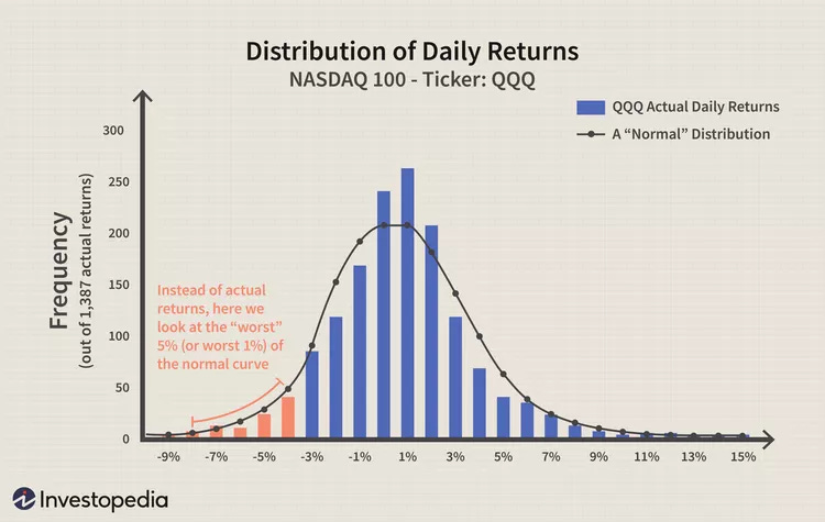
VaR commonly assumes that financial returns follow a normal distribution, which is often an inaccurate representation in real-world financial markets.
Many financial returns exhibit skewness and kurtosis, indicating fat tails and asymmetry. Consequently, VaR may underestimate the probability of extreme losses, which frequently occur in the tail regions of the distribution (Taleb, 2007).
Failure to Specify Loss Beyond the VaR:
While VaR provides an estimate of the maximum loss at a given confidence level, it fails to indicate the magnitude of potential losses if events surpass the VaR threshold. This limitation becomes particularly problematic during severe market downturns.
In such situations, an alternative measure called Conditional VaR (CVaR) proves more useful as it calculates the expected loss given that the VaR threshold has been exceeded, offering a more comprehensive risk estimate (Acerbi & Tasche, 2002).
Lack of Subadditivity:
Ideally, the combined VaR of two portfolios should be equal to or less than the sum of their individual VaRs, assuming diversification benefits. However, VaR lacks the property of subadditivity, which diminishes its reliability as a risk measurement tool for diversified portfolios (Artzner et al., 1999).
2008 Financial Crisis
The 2008 financial crisis served as a wake-up call, exposing the limitations of VaR. Many financial institutions relying on VaR models were ill-prepared for the extreme events of the crisis. With VaR models predominantly leveraging short-term historical data, they failed to accurately predict and account for the severity of the crisis, leading to substantial losses (Danielsson, 2011).
By recognizing and understanding the pitfalls and controversies associated with VaR, financial professionals can better assess its limitations and explore alternative risk measurement approaches to ensure more accurate risk management.
References
Acerbi, C., & Tasche, D. (2002). On the coherence of Expected Shortfall. Journal of Banking & Finance, 26(7), 1487-1503.
Artzner, P., Delbaen, F., Eber, J. M., & Heath, D. (1999). Coherent measures of risk. Mathematical finance, 9(3), 203-228.
Danielsson, J. (2011). Financial risk forecasting: The theory and practice of forecasting market risk with implementation in R and Matlab. John Wiley & Sons.
Jorion, P. (2007). Value at Risk: the new benchmark for managing financial risk. McGraw-Hill.
Linsmeier, T. J., & Pearson, N. D. (2000). Value at Risk. Financial Analysts Journal, 56(2), 47-67.
Taleb, N. N. (2007). The black swan: The impact of the highly improbable (Vol. 2). Random House.

