
Behavioral Finance: Understanding the Psychology Behind Investment Decisions
 In my years of working in finance, one thing has become abundantly clear: human emotions and cognitive biases play a significant role in financial decision-making. Traditional financial theories often assume investors act rationally, but my experience tells a different story.
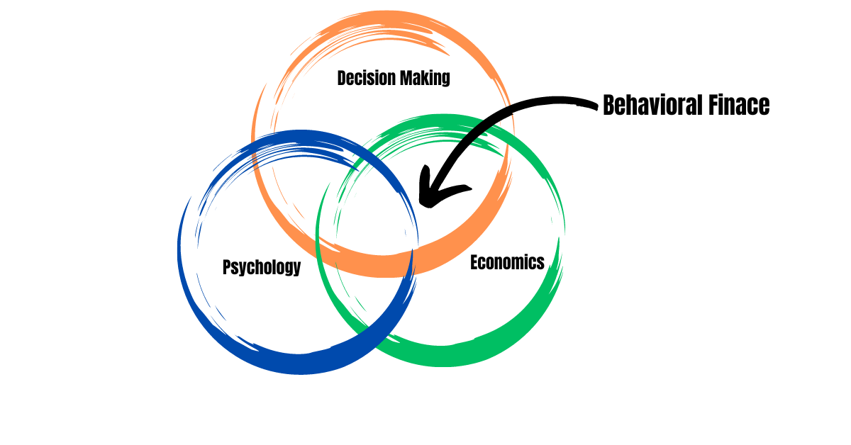
Behavioral finance, an interdisciplinary field that combines insights from psychology, sociology, and traditional finance, offers a more nuanced understanding of how individuals and markets behave.
I’ve seen firsthand how acknowledging these psychological factors can lead to better investment outcomes. In this article, I’ll share what I’ve learned about behavioral finance, its historical development, and its implications for investors. By understanding the psychological underpinnings of financial decisions, we can all strive to make more informed and rational choices.
What is Behavioral Finance?
Behavioral finance delves into how psychological factors influence financial decisions and, by extension, financial markets. It challenges the traditional notion that markets are always efficient and that investors always act rationally. From my perspective, this field has been a game-changer in understanding why people often make irrational financial choices.
Key concepts in behavioral finance include cognitive biases, heuristics, and prospect theory. These ideas help explain why we sometimes deviate from what traditional economic theories would predict.
For instance, cognitive biases are systematic errors in thinking that can lead to poor decision-making. Heuristics are mental shortcuts we use to make decisions quickly, which can sometimes lead us astray. Prospect theory, developed by Daniel Kahneman and Amos Tversky, describes how we make decisions under risk and uncertainty, often in ways that defy logic.
History of Behavioral Finance
The journey of behavioral finance began in the mid-20th century and gained momentum in the 1970s and 1980s. It’s fascinating to see how the field has evolved over the years.
In the early days, pioneers like Herbert Simon and Daniel Ellsberg laid the groundwork. Simon introduced “bounded rationality” in 1955, suggesting that our decision-making is limited by the information we have, our cognitive capabilities, and time constraints. Ellsberg’s paradox, presented in 1960, showed that people often prefer known risks over unknown ones, even if the known risk is less favorable.
The 1970s were a turning point. Daniel Kahneman and Amos Tversky’s 1974 paper introduced cognitive biases in decision-making, and their 1979 Prospect Theory challenged the Expected Utility Theory.
The 1980s and 1990s saw figures like Richard Thaler and Robert Shiller questioning the Efficient Market Hypothesis and providing evidence of market inefficiencies due to investor psychology.
From the 2000s to the present, behavioral finance has gained mainstream acceptance, with Nobel Prizes awarded to Kahneman in 2002 and Thaler in 2017. Today, behavioral finance influences policy-making, investment strategies, and financial product design.
Key Concepts in Behavioral Finance
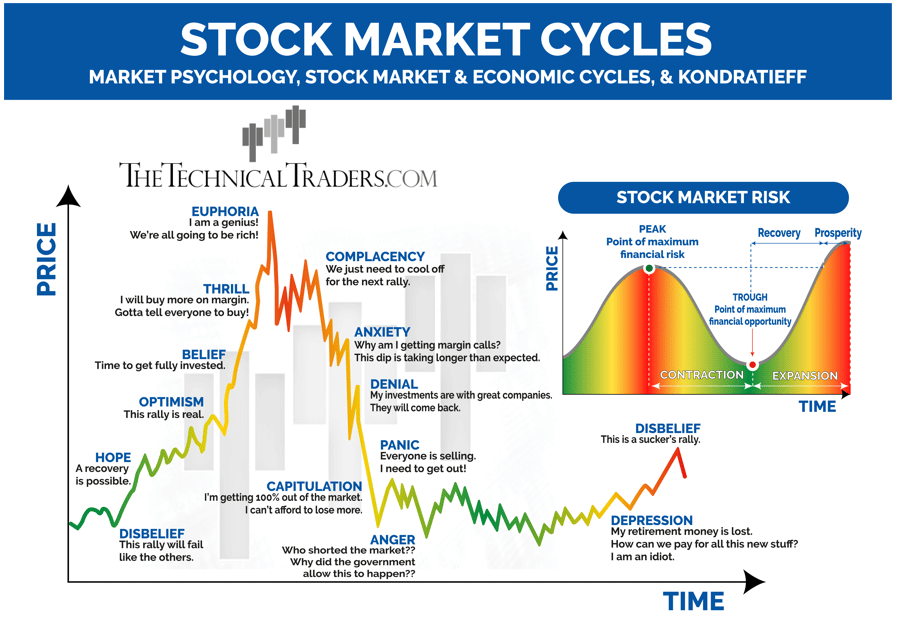
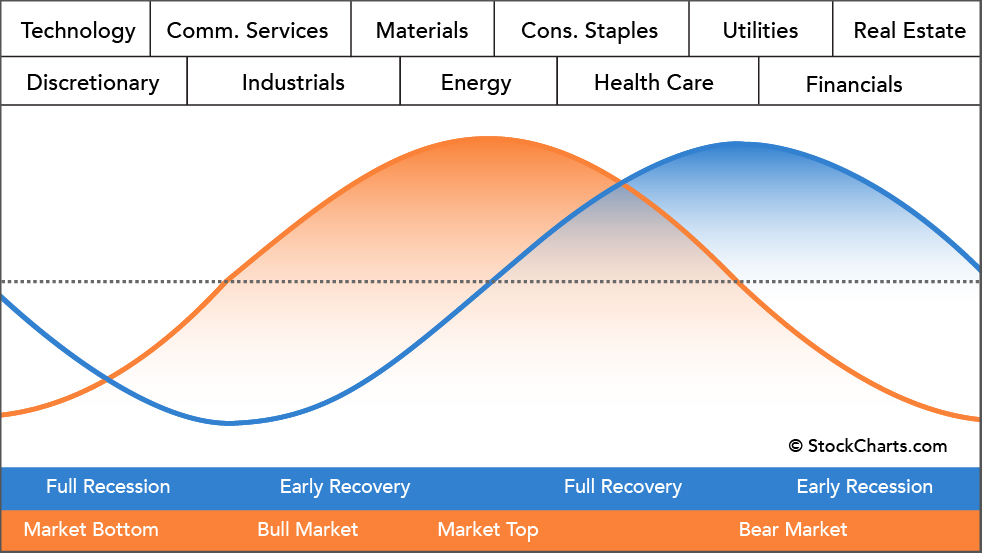
source: thetechincaltraders.com
Cognitive Biases:
Cognitive biases are systematic errors in thinking that can lead to poor decision-making. Some common ones in investing include:
- Confirmation Bias: Seeking out information that confirms existing beliefs while ignoring contradictory evidence.
- Anchoring Bias: Relying too heavily on the first piece of information encountered.
- Overconfidence Bias: Overestimating one’s own abilities or the accuracy of one’s predictions.
- Loss Aversion: Preferring to avoid losses over acquiring equivalent gains.
Heuristics:
Heuristics are mental shortcuts we use to make decisions quickly. While useful sometimes, they can lead to errors. Examples include:
- Availability Heuristic: Judging the probability of an event based on how easily examples come to mind.
- Representativeness Heuristic: Making judgments based on how similar something is to a known prototype or stereotype.
Prospect Theory:
Prospect Theory, developed by Kahneman and Tversky, describes how we make decisions under risk and uncertainty. Key aspects include:
Reference Point: Evaluating gains and losses relative to a reference point.
Loss Aversion: Feeling losses more strongly than equivalent gains.
Diminishing Sensitivity: The impact of gains or losses diminishes as their magnitude increases.
Market Anomalies:
Behavioral finance helps explain various market anomalies that traditional finance theories struggle to account for, such as:
- The Equity Premium Puzzle: Stocks have historically provided much higher returns than bonds, beyond what their higher risk can explain.
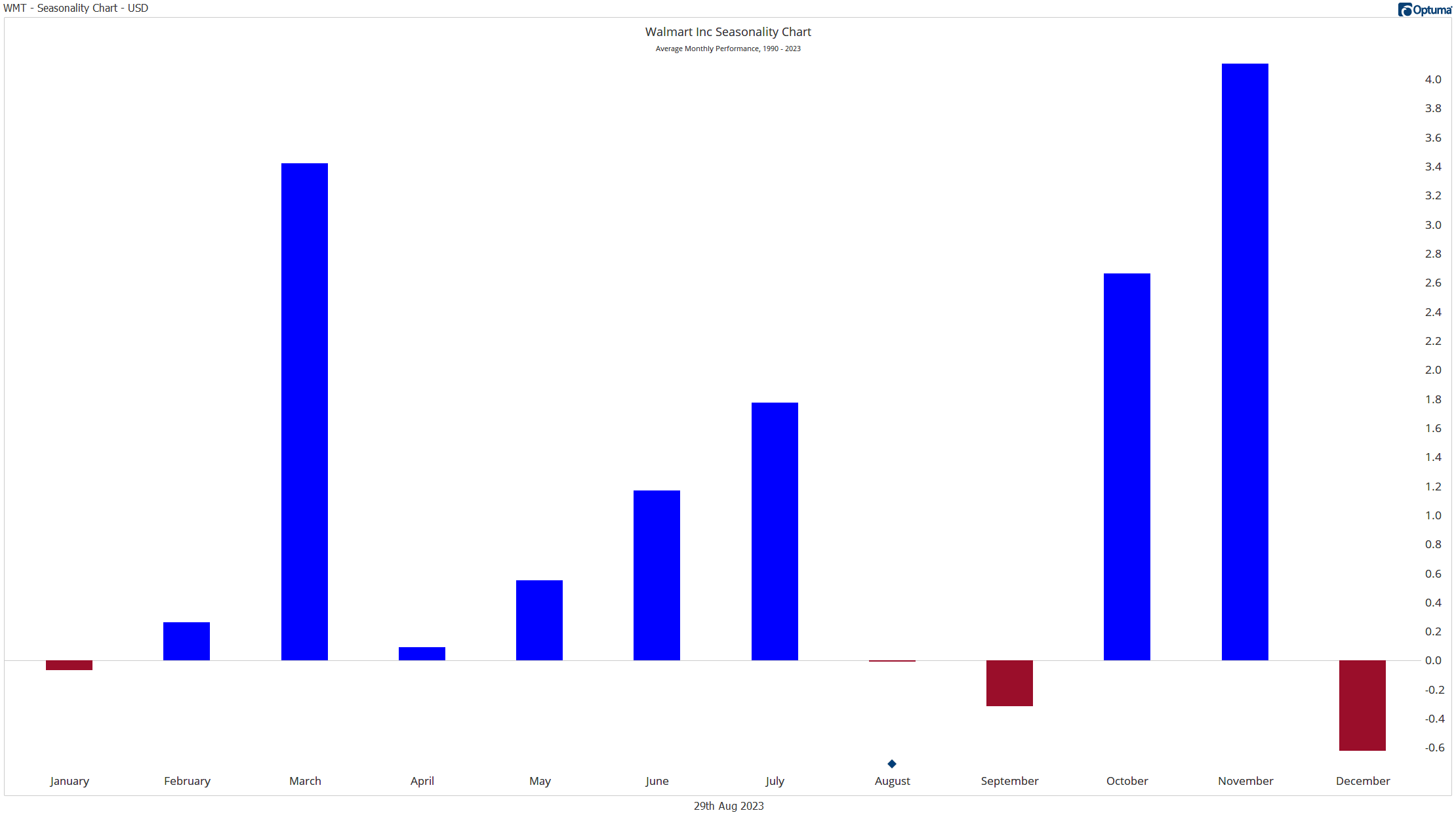
- The January Effect: Stock prices tend to rise in January more than in other months.
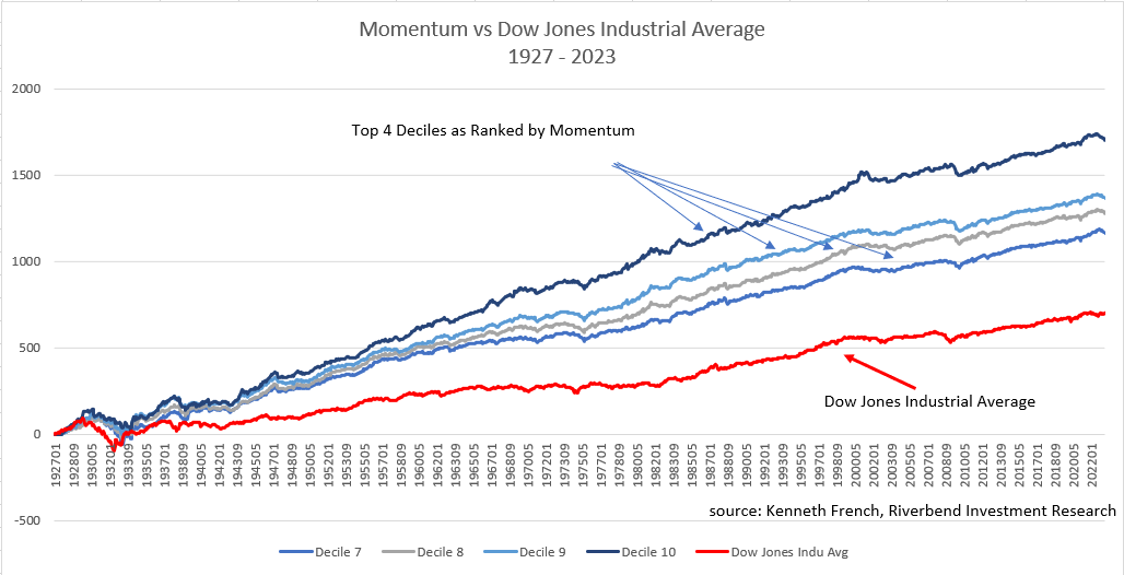
- Momentum Effect: Assets that have performed well in the recent past tend to continue performing well in the near future.
Implications for Investors
Understanding behavioral finance can have significant implications for investors:
Improved Decision-Making:
Recognizing cognitive biases and emotional influences can help investors make more rational decisions.
For example, being aware of confirmation bias can encourage seeking diverse perspectives and challenging one’s own assumptions.
Risk Management:
Insights from behavioral finance can help investors better understand and manage risk. Recognizing loss aversion can help avoid panic selling during market downturns.
Portfolio Construction:
Behavioral tendencies can inform portfolio construction strategies. For instance, using dollar-cost averaging can mitigate the impact of market timing biases.
Market Inefficiencies:
Behavioral finance suggests that markets may not always be efficient, creating opportunities for skilled investors to exploit mispricings.
Financial Product Design:
Insights from behavioral finance have led to new financial products and services, like robo-advisors that help automate investment decisions and reduce emotional biases.
Policy Implications:
Behavioral finance has influenced policy-making, leading to initiatives like automatic enrollment in retirement savings plans to overcome inertia and procrastination biases.
Case Study: The Dot-Com Bubble
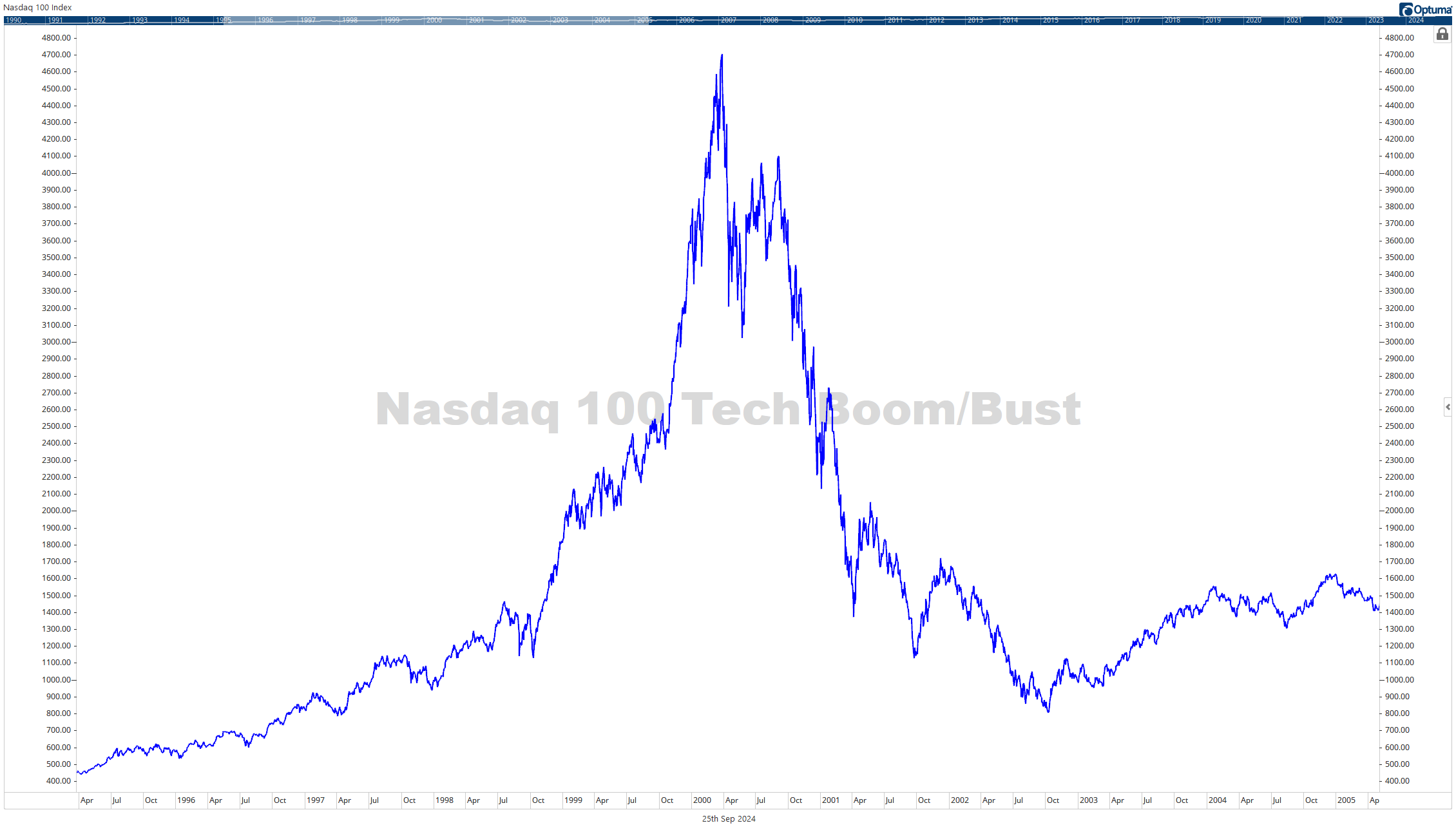
The dot-com bubble of the late 1990s and early 2000s offers a compelling example of behavioral finance principles in action. During this period, investors exhibited several cognitive biases:
- Overconfidence: Overestimating their ability to pick winning stocks in the new internet sector.
- Herding: Following suit as more people invested in tech stocks, creating a self-reinforcing cycle.
- Representativeness: Assuming all internet companies would be successful based on a few high-profile successes.
The result was a massive bubble in technology stocks, followed by a painful crash. This episode highlights the importance of understanding and managing behavioral biases in investing.
Conclusion:
Behavioral finance has revolutionized our understanding of financial markets and decision-making. By acknowledging the role of psychology in financial behavior, it provides a more nuanced and realistic view of how individuals and markets operate.
For investors, the insights from behavioral finance offer valuable tools for improving decision-making, managing risk, and potentially achieving better investment outcomes.
However, it’s important to note that while behavioral finance provides valuable insights, it doesn’t offer a perfect solution to all investment challenges.
Markets are complex systems influenced by numerous factors, and human behavior is just one piece of the puzzle. Nonetheless, by incorporating behavioral finance principles into their investment approach, investors can potentially make more informed decisions and avoid common pitfalls.
As the field continues to evolve, it promises to yield further insights that can help investors navigate the complexities of financial markets. By staying informed about behavioral finance research and applying its principles, investors can strive to become more rational, disciplined, and successful in their financial endeavors.
Sources:
- Kahneman, D., & Tversky, A. (1979). Prospect Theory: An Analysis of Decision under Risk. Econometrica
- Thaler, R. H. (2015). Misbehaving: The Making of Behavioral Economics. W. W. Norton & Company.
- Shiller, R. J. (2003). From Efficient Markets Theory to Behavioral Finance. Journal of Economic Perspectives
- De Bondt, W. F., & Thaler, R. (1985). Does the Stock Market Overreact? The Journal of Finance
- Barberis, N., & Thaler, R. (2003). A Survey of Behavioral Finance. Handbook of the Economics of Finance
- Tversky, A., & Kahneman, D. (1974). Judgment under Uncertainty: Heuristics and Biases. Science
- Fama, E. F. (1970). Efficient Capital Markets: A Review of Theory and Empirical Work. The Journal of Finance
- Statman, M. (2014). Behavioral Finance: Finance with Normal People. Borsa Istanbul Review
- Shefrin, H. (2000). Beyond Greed and Fear: Understanding Behavioral Finance and the Psychology of Investing. Oxford University Press
- Pompian, M. M. (2011). Behavioral Finance and Wealth Management: How to Build Optimal Portfolios That Account for Investor Biases. John Wiley & Sons
- Baker, H. K., & Nofsinger, J. R. (2010). Behavioral Finance: Investors, Corporations, and Markets. John Wiley & Sons
- Hirshleifer, D. (2015). Behavioral Finance. Annual Review of Financial Economics
- Sewell, M. (2007). Behavioural Finance. University of Cambridge
- Ricciardi, V., & Simon, H. K. (2000). What is Behavioral Finance? Business, Education & Technology Journal
- Ritter, J. R. (2003). Behavioral Finance. Pacific-Basin Finance Journal
- Statman, M. (1999). Behavioral Finance: Past Battles and Future Engagements. Financial Analysts Journal
- Daniel, K., Hirshleifer, D., & Subrahmanyam, A. (1998). Investor Psychology and Security Market Under‐ and Overreactions. The Journal of Finance
- Barberis, N., Shleifer, A., & Vishny, R. (1998). A Model of Investor Sentiment. Journal of Financial Economics
- Shleifer, A. (2000). Inefficient Markets: An Introduction to Behavioral Finance. Oxford University Press
- Lo, A. W. (2004). The Adaptive Markets Hypothesis: Market Efficiency from an Evolutionary Perspective. Journal of Portfolio Management
 Exxon 1970-1979. Source: Macrotrends
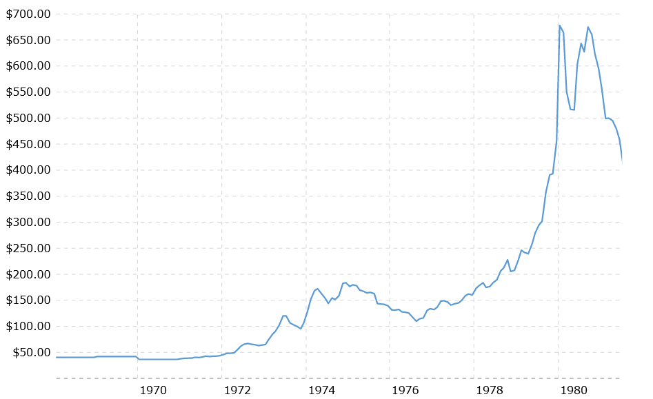
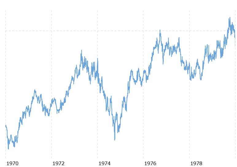
 Source: JPMorgan
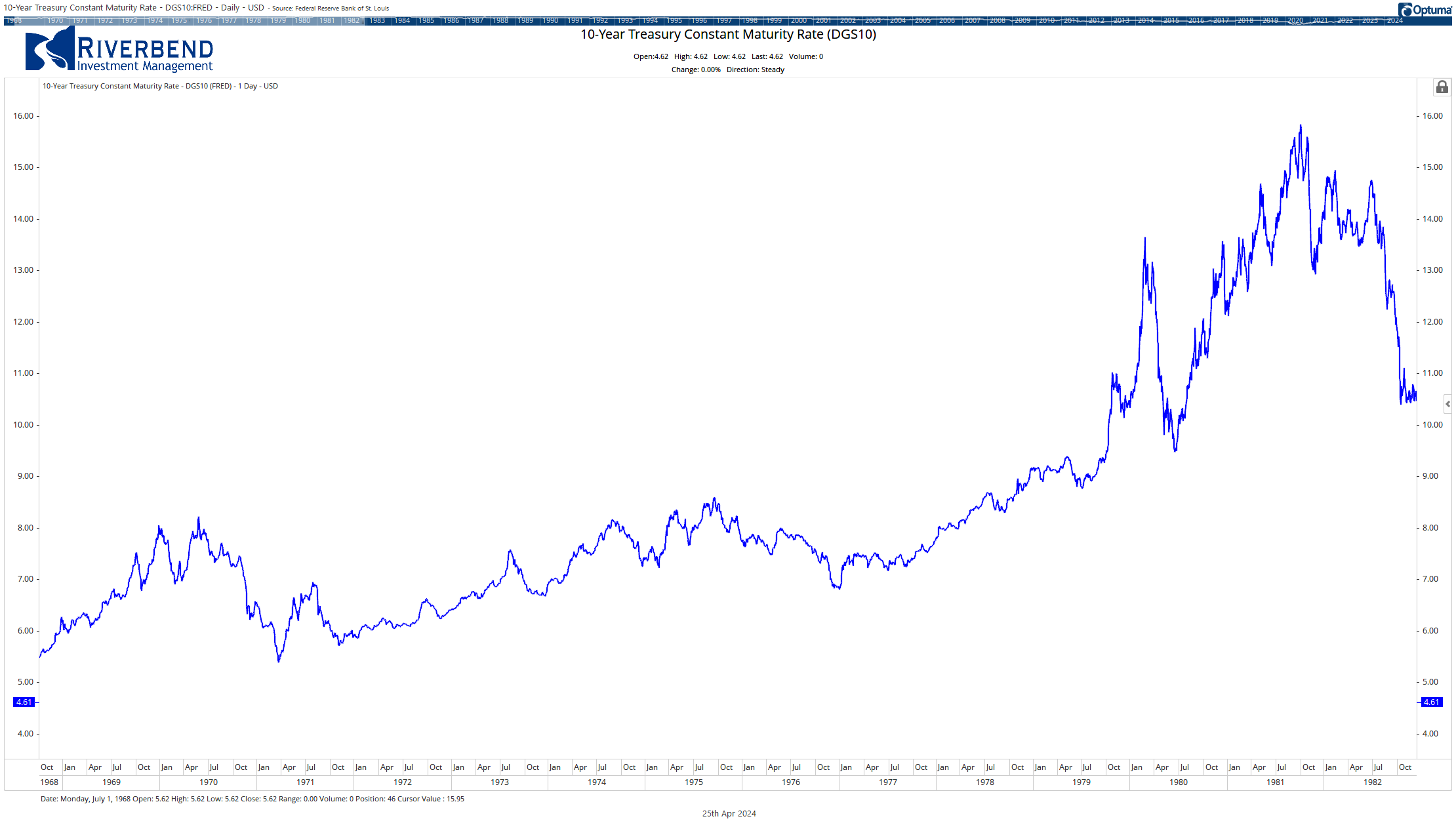
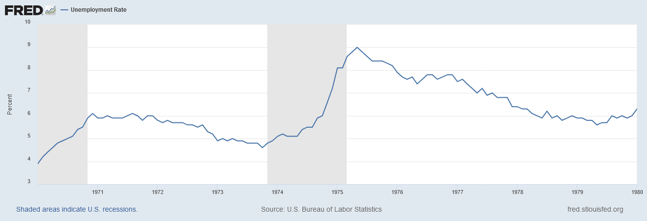
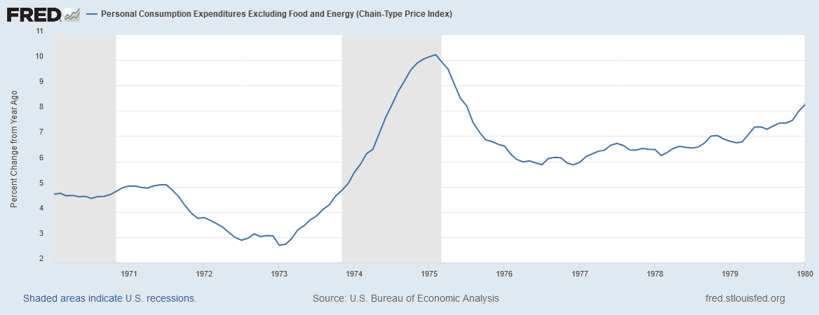
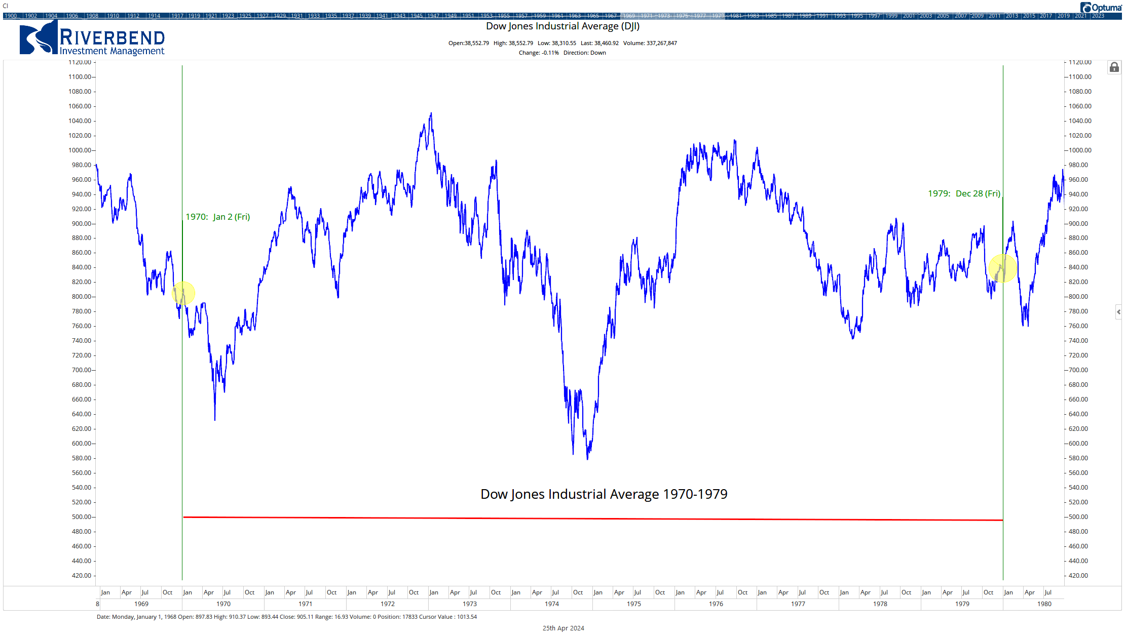
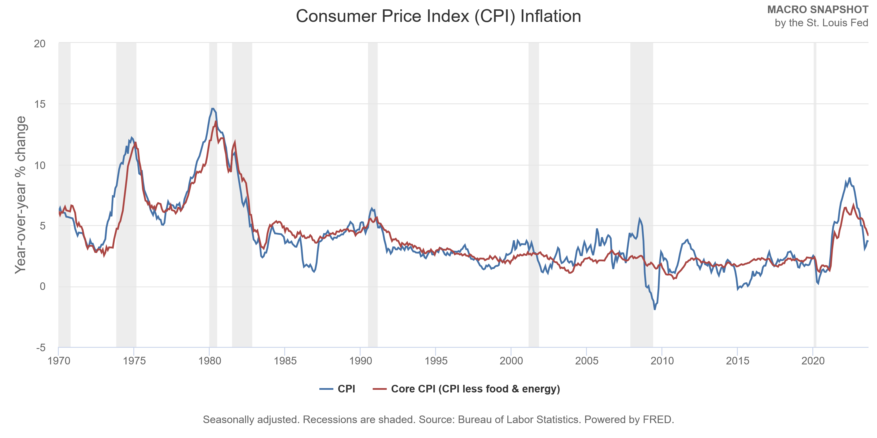
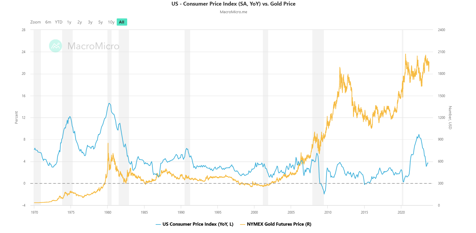
 Source: Fred, Riverbend Investment Management

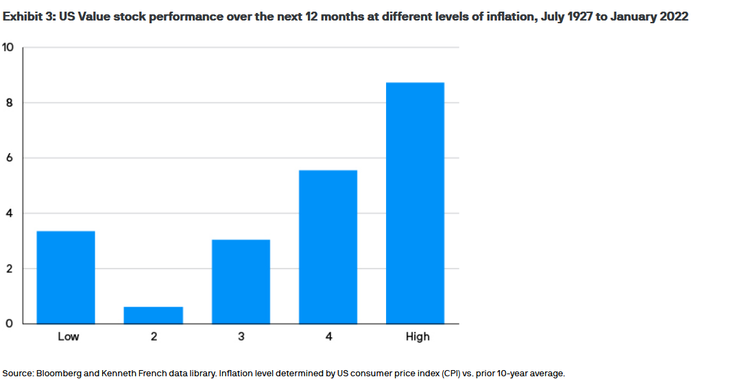
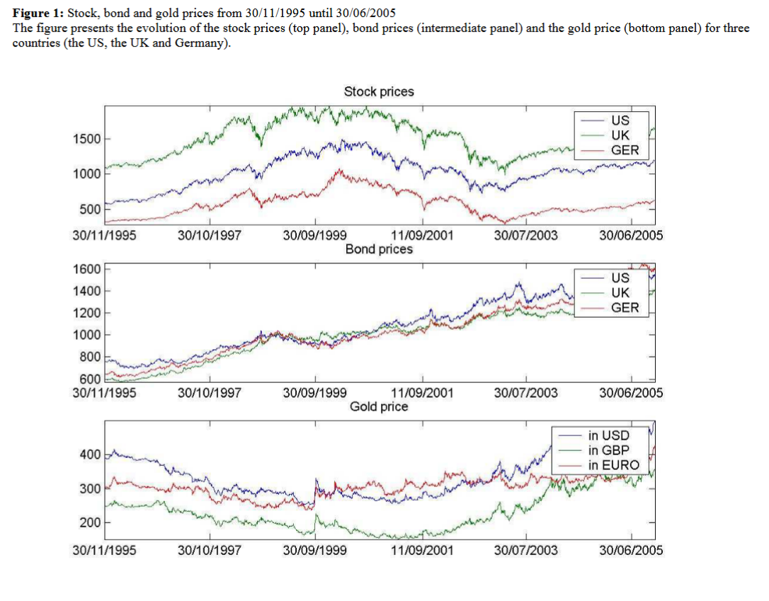 Source: “Is Gold a Hedge or a Safe Haven? An Analysis of Stocks, Bonds, and Gold”
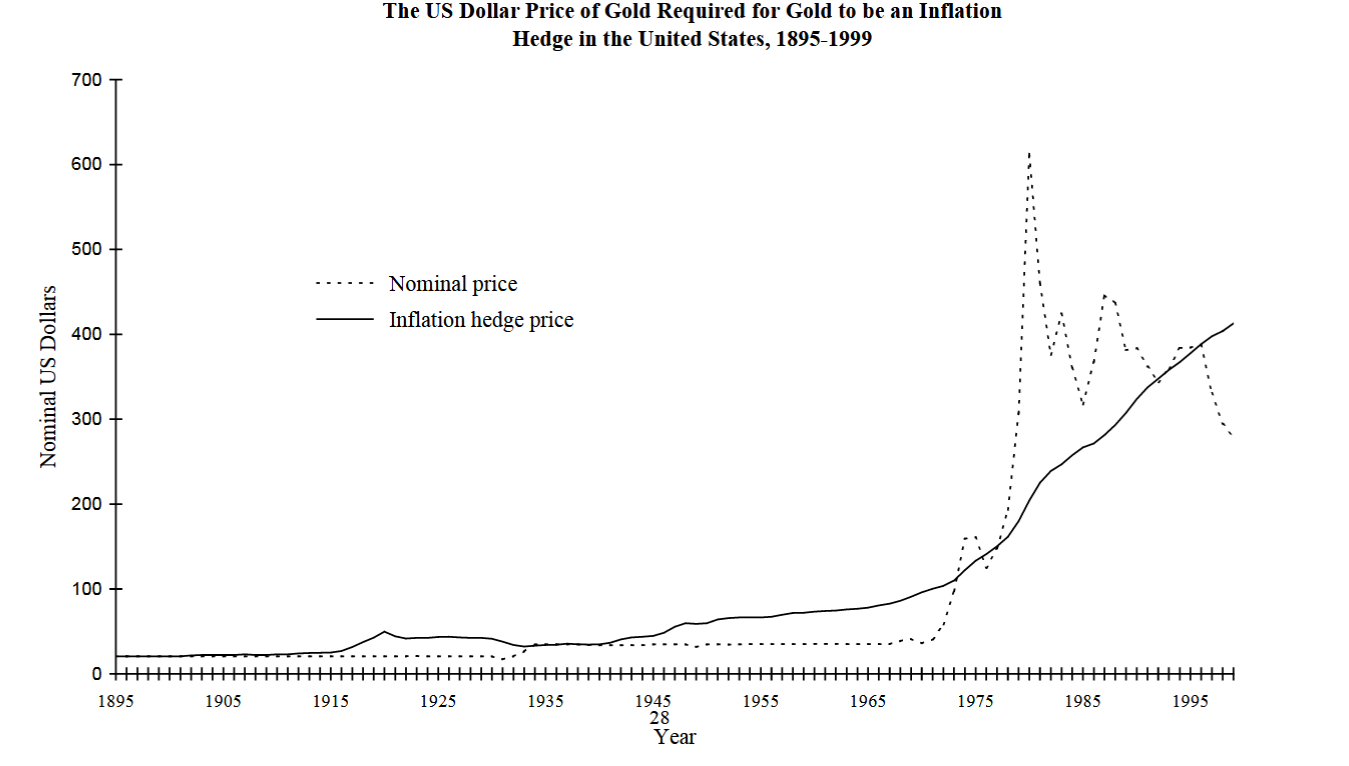 Source: “Gold as an Inflation Hedge”